Five Spot Pattern Single Phase#

Author: Zakariya Abugrin | Date: May 2025

Introduction#

This tutorial shows how to create a simple regular cartesian grid with a single phase fluid and a five-spot wells’ pattern. The user can use this tutorial to test the change in pressure distribution based on the rock (i.e. grid) and fluid properties or using a different wells’ pattern.

*the code used to generate this gif image is shown in Save simulation run as gif section below.

Import `reservoirflow`#

We start with importing reservoirflow as rf. The abbreviation rf refers to reservoirflow where all modules under this library can be accessed. rf is also used throughout the API documentation. We recommend our users to stick with this convention.

import reservoirflow as rf

print(rf.__version__)

0.1.0b3

static = True
notebook = True

Both static and notebook are set to True to produce images for this notebook. For an interactive visualization in your local machine, set both arguments to False. To allow for interactive visualizations in Colab, set only static=False and keep notebook=True.

rf.utils.pyvista.set_mode("dark")

By default, "dark" mode is used with a black background. You can change to "light" mode using rf.utils.pyvista.set_mode() function.

Define a regular cartesian grid#

We start with defining the grid model which represents the rock geometry and properties using grids module. Currently, only RegularCartesian grid models are supported. In the near future, Radial and IrregularCartesian models will be added.

grid = rf.grids.RegularCartesian(
    nx=7,
    ny=7,
    nz=3,
    dx=200,
    dy=200,
    dz=40,
    phi=0.30,
    kx=1,
    ky=1,
    kz=1,
    comp=1e-6,
    unit="field",
)

Note

Note that field units are used in this tutorial. For more information about selecting a unit system or what units or factors are used for each property, see Units & Factors.

The grid object can be shown using show() method. Argument label can be used to show cells id or other properties. For more information, check RegularCartesian.

grid.show(
    label="id",
    boundary=True,
    static=static,
    notebook=notebook,
)

../../_images/9e11f8e5b6279ce6ef2550df0454f972e5eaa7622f12264a96d865e76d2bc2e2.png

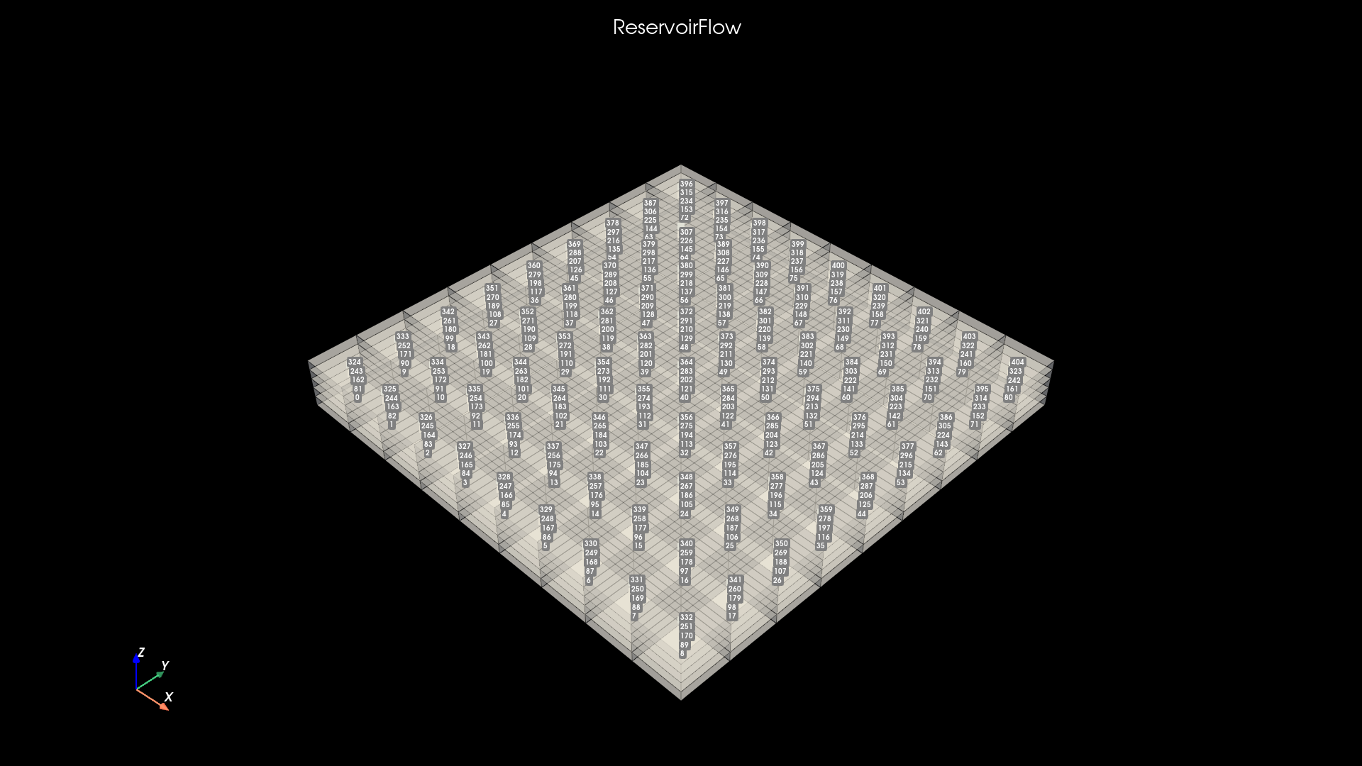
Note

Cells are given an id based on natural order starting form the bottom left corner, see grid.cells_id. Cells id increase in x from left to right, in y from front to back, and in z from bottom to top. Boundaries are also counted. You can use the cell id to access its properties, or add a well in that location as shown in Add wells section below.

Define a single phase compressible fluid#

After defining the grid model, we can use the fluids module to define a fluid. A single phase fluid can be defined using SinglePhase class which accepts arguments such s viscosity (mu), formation volume factor (B), density (rho), compressibility (comp) etc. For more information, check SinglePhase.

fluid = rf.fluids.SinglePhase(
    mu=0.5,
    B=1,
    rho=50,
    comp=1e-5,
    unit="field",
)

Create a reservoir simulation model#

To construct a reservoir simulation model, both fluid and grid objects are required as input arguments in models module. In addition, you can also define the initial reservoir pressure (pi), time step duration (dt), start date etc. For more information, check models. Currently, only BlackOil models are supported. In the future, more advanced models will be added such as Compositional or Thermal.

model = rf.models.BlackOil(
    grid=grid,
    fluid=fluid,
    pi=3000,
    dt=1,
    start_date="01.01.2000",
    unit="field",
)

Define boundary conditions#

If you start the simulation run without defining a boundary condition, then all boundaries are set to zero flow rate. To define a boundary condition, you can use set_boundaries() method where you specify the boundary condition as dictionary where keys are cells id and values are tuple of (“cond”, value). For example, a constant zero rate boundary condition in cell_id=0 can be set as model.set_boundaries({0: ("rate", 0)}).

Below we set all the boundaries cells to zero rate (default behavior).

model.set_boundaries({i: ("rate", 0) for i in grid.get_boundaries("id", fmt="array")})

Add wells#

To make a five spot pattern, single cell wells are used to add wells to specific cells as following:

Injection wells#

4 injectors: 182, 186, 218, 222

for cell_id in [182, 186, 218, 222]:
    model.set_well(cell_id=cell_id, pwf=3500, s=0, r=3.5)

Note

Since the bottom hole flowing pressure (BHFP or pwf) is higher than the initial reservoir pressure, then these wells will have an injection rates (i.e. a positive flow rate means additional fluid is injected into the reservoir). This might not be the expected behavior in reservoir simulation and this might be reversed in the future where injection rates will be expressed as a negative rate (depends on the users’ feedback). Feel free to comment on this.

Production well#

1 producer: 202

model.set_well(
    cell_id=202,
    pwf=1000,
    s=0,
    r=3.5,
)

Note

In this case, pwf is lower than the initial reservoir pressure, which will lead to a production rates (i.e. a negative flow rate means a fluid is produced from the reservoir).

Compile the model#

Before you can run the model, you need to compile a solution for it. By compiling a solution, you actually decide the solution you want to use for your model. Interestingly, reservoirflow provides multiple solutions for the same model based on your configuration.

Hint

Compiling solutions is the most interesting idea introduced in reservoirflow which allows to solve the same model using different solutions so we can compare them with each other and/or combine them together.

Currently, a numerical solution based on Finite-Difference-Method (FDM) is available. You can read more about the available solution in the solutions. Below, we compile our model using a numerical solution using FDM.

model.compile(stype="numerical", method="FDM", sparse=False)

[info] FDM was assigned as model.solution.

Attention

A model can not be run until it is complied. Methods such as solve() and run() will be functioning only after the model is compiled.

Run the model with 40 time steps#

To run the simulation model, use run() method as shown below. Here, you can set the number of time steps based on nsteps argument. Note that each time step will have a time duration as defined by dt argument when the model was constructed.

There are two modes available run the model based on vectorize argument, True means vectorized and False means symbolized. In addition, you can also select a solver which can be direct, iterative, or neurical. Developing solvers based on neural-networks is also a new idea introduced by reservoirflow.

model.run(
    nsteps=40,
    vectorize=True,
    isolver=None,
)

[info] Simulation run started: 40 timesteps.
[info] Simulation run of 40 steps finished in 0.13 seconds.
[info] Material Balance Error: 1.3280299082651936e-10.

Visualize the simulation run in 3D show#

You can interactively show the simulation run in a 3D show using show() method. There is a lot of functionality here. For interactive visualization, set static and notebook to False. For more information, check the BlackOil.show().

Note

Here, boundaries are also added (boundary=True) but they appear in a gray color. That is because boundaries are defined as a zero flow rate where pressures are undefined (i.e. np.nan). If boundary conditions were set to constant pressures, values will appear based on the defined color map.

model.show(
    prop="pressures",
    boundary=True,
    cmap="Blues",
    static=static,
    notebook=notebook,
)

../../_images/fe79e85ba16a0e6d3fb6acc502706d33d9c7b596d588acafd81d99489d94e568.png

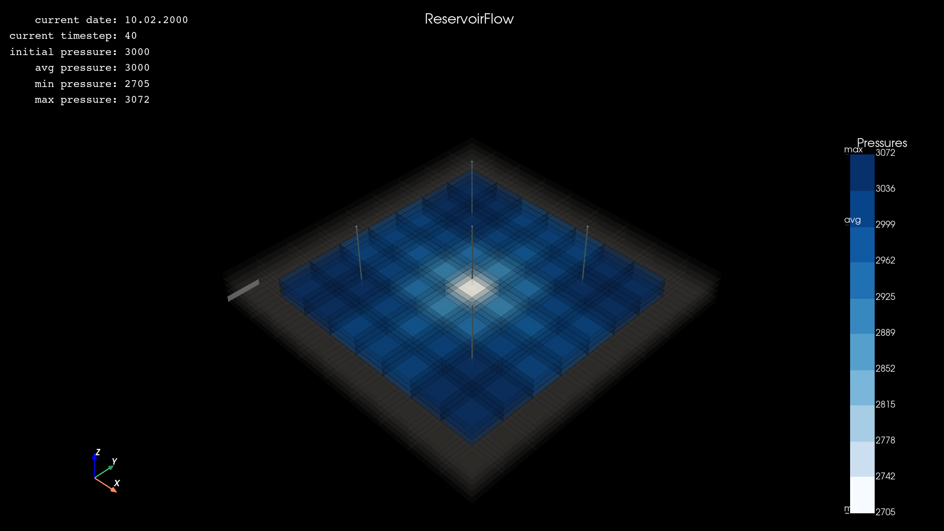
Tip

Use the color maps names as str with cmap argument. Matplotlib color maps are supported, for more color maps, check Choosing Colormaps in Matplotlib. In the above image, cmap="Blues" was used. In Save simulation run as gif section below, cmap="tab10" was used instead.

Show results as a pandas `DataFrame`#

The results of the Simulation run can be accessed as a pandas DateFrame using get_df() method. You can select columns and scale values. For more information, check BlackOil.get_df().

df = model.get_df(columns=["time", "date", "wells"], units=True).round()
df

	Time [days]	Date [d.m.y]	Qw182 [stb/day]	Qw186 [stb/day]	Qw218 [stb/day]	Qw222 [stb/day]	Qw202 [stb/day]	Pwf182 [psia]	Pwf186 [psia]	Pwf218 [psia]	Pwf222 [psia]	Pwf202 [psia]
Step
0	0	01.01.2000	0.0	0.0	0.0	0.0	0.0	3000.0	3000.0	3000.0	3000.0	3000.0
1	1	02.01.2000	55.0	55.0	55.0	55.0	-222.0	3500.0	3500.0	3500.0	3500.0	1000.0
2	2	03.01.2000	54.0	54.0	54.0	54.0	-217.0	3500.0	3500.0	3500.0	3500.0	1000.0
3	3	04.01.2000	53.0	53.0	53.0	53.0	-213.0	3500.0	3500.0	3500.0	3500.0	1000.0
4	4	05.01.2000	53.0	53.0	53.0	53.0	-210.0	3500.0	3500.0	3500.0	3500.0	1000.0
5	5	06.01.2000	52.0	52.0	52.0	52.0	-208.0	3500.0	3500.0	3500.0	3500.0	1000.0
6	6	07.01.2000	52.0	52.0	52.0	52.0	-207.0	3500.0	3500.0	3500.0	3500.0	1000.0
7	7	08.01.2000	51.0	51.0	51.0	51.0	-205.0	3500.0	3500.0	3500.0	3500.0	1000.0
8	8	09.01.2000	51.0	51.0	51.0	51.0	-204.0	3500.0	3500.0	3500.0	3500.0	1000.0
9	9	10.01.2000	51.0	51.0	51.0	51.0	-203.0	3500.0	3500.0	3500.0	3500.0	1000.0
10	10	11.01.2000	51.0	51.0	51.0	51.0	-203.0	3500.0	3500.0	3500.0	3500.0	1000.0
11	11	12.01.2000	50.0	50.0	50.0	50.0	-202.0	3500.0	3500.0	3500.0	3500.0	1000.0
12	12	13.01.2000	50.0	50.0	50.0	50.0	-201.0	3500.0	3500.0	3500.0	3500.0	1000.0
13	13	14.01.2000	50.0	50.0	50.0	50.0	-201.0	3500.0	3500.0	3500.0	3500.0	1000.0
14	14	15.01.2000	50.0	50.0	50.0	50.0	-200.0	3500.0	3500.0	3500.0	3500.0	1000.0
15	15	16.01.2000	50.0	50.0	50.0	50.0	-200.0	3500.0	3500.0	3500.0	3500.0	1000.0
16	16	17.01.2000	50.0	50.0	50.0	50.0	-200.0	3500.0	3500.0	3500.0	3500.0	1000.0
17	17	18.01.2000	50.0	50.0	50.0	50.0	-199.0	3500.0	3500.0	3500.0	3500.0	1000.0
18	18	19.01.2000	50.0	50.0	50.0	50.0	-199.0	3500.0	3500.0	3500.0	3500.0	1000.0
19	19	20.01.2000	50.0	50.0	50.0	50.0	-199.0	3500.0	3500.0	3500.0	3500.0	1000.0
20	20	21.01.2000	50.0	50.0	50.0	50.0	-199.0	3500.0	3500.0	3500.0	3500.0	1000.0
21	21	22.01.2000	50.0	50.0	50.0	50.0	-198.0	3500.0	3500.0	3500.0	3500.0	1000.0
22	22	23.01.2000	50.0	50.0	50.0	50.0	-198.0	3500.0	3500.0	3500.0	3500.0	1000.0
23	23	24.01.2000	50.0	50.0	50.0	50.0	-198.0	3500.0	3500.0	3500.0	3500.0	1000.0
24	24	25.01.2000	50.0	50.0	50.0	50.0	-198.0	3500.0	3500.0	3500.0	3500.0	1000.0
25	25	26.01.2000	50.0	50.0	50.0	50.0	-198.0	3500.0	3500.0	3500.0	3500.0	1000.0
26	26	27.01.2000	50.0	50.0	50.0	50.0	-198.0	3500.0	3500.0	3500.0	3500.0	1000.0
27	27	28.01.2000	50.0	50.0	50.0	50.0	-198.0	3500.0	3500.0	3500.0	3500.0	1000.0
28	28	29.01.2000	49.0	49.0	49.0	49.0	-197.0	3500.0	3500.0	3500.0	3500.0	1000.0
29	29	30.01.2000	49.0	49.0	49.0	49.0	-197.0	3500.0	3500.0	3500.0	3500.0	1000.0
30	30	31.01.2000	49.0	49.0	49.0	49.0	-197.0	3500.0	3500.0	3500.0	3500.0	1000.0
31	31	01.02.2000	49.0	49.0	49.0	49.0	-197.0	3500.0	3500.0	3500.0	3500.0	1000.0
32	32	02.02.2000	49.0	49.0	49.0	49.0	-197.0	3500.0	3500.0	3500.0	3500.0	1000.0
33	33	03.02.2000	49.0	49.0	49.0	49.0	-197.0	3500.0	3500.0	3500.0	3500.0	1000.0
34	34	04.02.2000	49.0	49.0	49.0	49.0	-197.0	3500.0	3500.0	3500.0	3500.0	1000.0
35	35	05.02.2000	49.0	49.0	49.0	49.0	-197.0	3500.0	3500.0	3500.0	3500.0	1000.0
36	36	06.02.2000	49.0	49.0	49.0	49.0	-197.0	3500.0	3500.0	3500.0	3500.0	1000.0
37	37	07.02.2000	49.0	49.0	49.0	49.0	-197.0	3500.0	3500.0	3500.0	3500.0	1000.0
38	38	08.02.2000	49.0	49.0	49.0	49.0	-197.0	3500.0	3500.0	3500.0	3500.0	1000.0
39	39	09.02.2000	49.0	49.0	49.0	49.0	-197.0	3500.0	3500.0	3500.0	3500.0	1000.0
40	40	10.02.2000	49.0	49.0	49.0	49.0	-197.0	3500.0	3500.0	3500.0	3500.0	1000.0

Save simulation run as gif#

You can save gif movie of the simulation run using save_gif() method. For more information, check the BlackOil.save_gif().

if not static:
    model.save_gif(
        prop="pressures",
        boundary=False,
        cmap="tab10",
        file_name="attachments/grid_animated.gif",
        window_size=rf.utils.pyvista.get_window_size("hd"),
    )

Tip

To save a gif movie of the simulation run, set static=False or just remove the first line and unindent.

Comments 💬#

Feel free to make a comment, ask a question, or share your opinion about this specific content. Please keep in mind the Commenting Guidelines ⚖.

Five Spot Pattern Single Phase#

Introduction#

Import reservoirflow#

Define a regular cartesian grid#

Define a single phase compressible fluid#

Create a reservoir simulation model#

Define boundary conditions#

Add wells#

Injection wells#

Production well#

Compile the model#

Run the model with 40 time steps#

Visualize the simulation run in 3D show#

Show results as a pandas DataFrame#

Save simulation run as gif#

Comments 💬#

Import `reservoirflow`#

Show results as a pandas `DataFrame`#